Benchmarking Guppy algorithms
on Bioinformatics, Nanopore, Guppy, Benchmark
ONT’s basecaller Guppy has recently been released to the masses. And with the announcement of the new “flip-flop” basecalling algorithm there is now the choice of two different algorithms for basecalling.
ONT has obviously been singing flip-flop’s praises, and understandably so, as the initial results look like a decent step up in read accuracy.
For an upcoming project I am going to be doing a lot of basecalling of Mycobacterium tuberculosis and given the project will involve assessing metrics heavily reliant on read accuracy I thought it best to invest some time in deciding which algorithm to go with. Another reason for my indecision came when I read a recent blog from Keith Robison which showed that maybe the new flip-flop algorithm doesn’t work well with organisms that have a higher GC content.
As M. tuberculosis has a GC content around 65% I thought it best to do a little benchmarking of the two basecalling algorithms first. Unfortunately for me, I couldn’t really rely on the results from Ryan Wick’s wonderful basecalling comparison due to the species he used, E. coli, having a roughly even GC content.
Note: Just before publishing this post Ryan released an updated version of the comparison as a preprint. In the test set there was one bacteria, Stenotrophomonas maltophilia, with a GC content similar to M. tuberculosis. Figure 2 in that paper shows flip-flop as having a higher read identity than the default Guppy algorithm.
What I will do here is walk through a small-scale basecalling algorithm comparison of the default Guppy algorithm and the flip-flop algorithm that comes as a config option with Guppy.
The data I am using to run this analysis was sequenced on an R9.4.1 flowcell. It was also a multiplexed run with 5 clinical samples of M. tuberculosis.
I’ll add in some code snippets for how I ran this analysis so you can recreate at home with your own data too. If you aren’t interested and just want to see some results then feel free to skip ahead.
Methods
Basecall
The only thing we need to change in order to use the flip-flop algorithm is to change the config file used.
Default config
cd Guppy_testing/normal
input=../fast5
output=basecalled_fastq/

guppy_basecaller --input_path "$input" \
    --save_path "$output" \
    --recursive \
    --verbose_logs \
    --worker_threads 32 \
    --config dna_r9.4.1_450bps.cfg
Basecalling took 120077.25 CPU seconds. As there are 1009917 reads total, that is approximately 505 reads/min.
Flip-flop config
cd Guppy_testing/flipflop
input=../fast5
output=basecalled_fastq/

guppy_basecaller --input_path "$input" \
    --save_path "$output" \
    --recursive \
    --verbose_logs \
    --worker_threads 32 \
    --config dna_r9.4.1_450bps_flipflop.cfg
Basecalling took 4051443 CPU seconds. As there are 1009917 reads total, that is approximately 15 reads/min.
At the time of writing this, I have not been able to run Guppy on the GPUs here. But once I have done that I will add the runtime figures for that too.
In terms of wall clock time, I ran the default config on 32 cores and it completed in 4.33 hours. For the flip-flop, I also ran it on 32 cores and it completed in 35.33 hours.
Barcode demultiplexing
As this is a 5x multiplexed sample I chose to use Ryan Wick’s Deepbinner tool for demultiplexing. From the results in the Deepbinner paper, and from my own personal testing, Deepbinner saves a lot more reads from the dreaded “unknown” bin.
Deepbinner classification
fast5_dir=../fast5
output=classification

deepbinner classify --native "$fast5_dir" > "$output"
I ran the deepbinner classification step on a GPU and it took 10 hours to classify all 1009917 reads - so approximately 1683 reads/min.
Deepbinner binning
Split the reads into separate fastq files for each barcode based on the classifications learned.
cd Guppy_testing/normal
classifications=../classification
out_dir=barcode_bins/
reads_dir=basecalled_fastq/

# combine all the fastq files into a single one
cat $(find $reads_dir -name '*.fastq') > tmp_reads.fastq

deepbinner bin \
    --classes "$classifications" \
    --reads tmp_reads.fastq \
    --out_dir "$out_dir"

rm tmp_reads.fastq
Do the same thing for Guppy_testing/flipflop.
Adapter trimming
Chop off adapter sequences using another of Ryan Wick’s tools, Porechop.
cd Guppy_testing/normal
outdir=barcode_bins/

# I only expect barcodes 1-5
for f in $(find barcode_bins/ -type f | grep -E 'barcode0[1-5].fastq.gz')
do
  name=$(basename $f)
  porechop --input "$f" \
          --output "$outdir"/"${name%%.*}".trimmed.fastq.gz \
          --discard_middle
done
Do the same thing for Guppy_testing/flipflop.
Map
The accuracy of the reads will be based on alignment to the reference genome. The alignment is done using minimap2.
cd Guppy_testing/normal
reference=../NC_000962.3.fa
outdir=mapped/
for f in $(find barcode_bins/ -name '*trimmed*')
do
  sample=$(basename ${f%%.*})
  output="$outdir"/"$sample".sorted.bam
  minimap2 -ax map-ont "$reference" "$f" | samtools sort -o "$output" -
done
Do the same thing for Guppy_testing/flipflop.
Plotting
I did some quality control plotting using a python package I developed called Pistis.
cd /hps/nobackup/research/zi/mbhall/Guppy_testing/normal
for i in {1..5}
do
  bam=mapped/barcode0"$i".sorted.bam
  reads=barcode_bins/barcode0"$i".trimmed.fastq.gz
  output=reports/barcode0"$i"_pistis.pdf
  pistis --fastq "$reads" --bam "$bam" \
      --output "$output" --downsample 0
done
Do the same thing for Guppy_testing/flipflop.
Results
Quality vs Read length
Probably the most startling thing for me initially was the difference in Phred quality scores the two algorithms were producing.
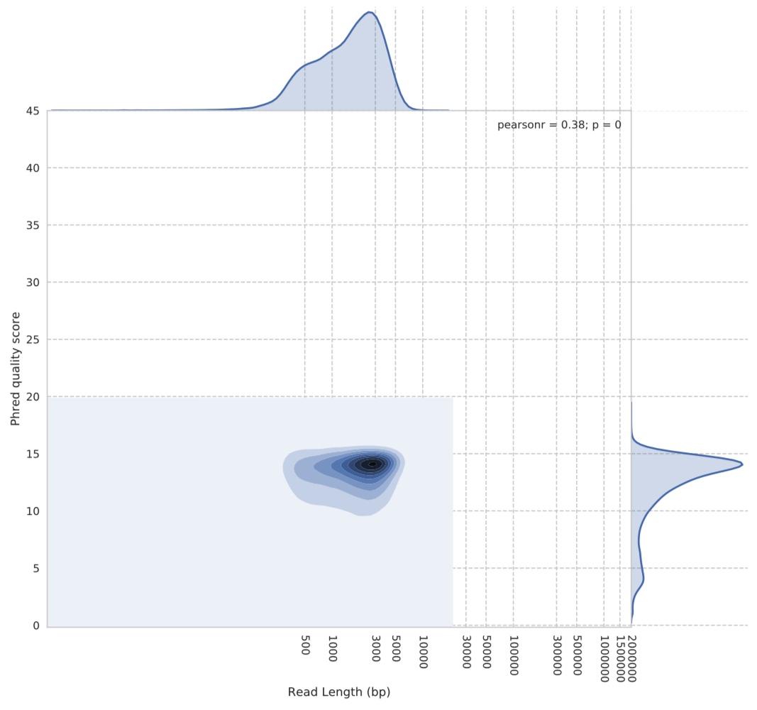 Figure 1: Guppy default basecalling algorithm quality vs read length. The y-axis shows the Phred quality score average for each read. The x-axis is the reads length in base pairs.
We can see from Figure 1 above that the Phred scores for the default algorithm are centred around 14. However, when we look at the same plot for the flip-flop algorithm (Figure 2), we see a very different story in terms of quality scores.
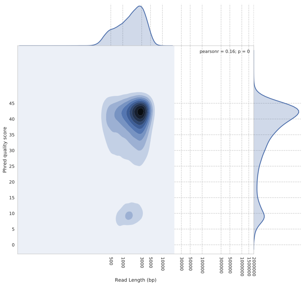 Figure 2: Guppy flip-flop basecalling algorithm quality vs read length. The y-axis shows the Phred quality score average for each read. The x-axis is the reads length in base pairs.
As you can see, flip-flop seems to rate itself very highly. The densest part of the kernel being around Phred score 42….yes, 42.
At the end of the day though, I don’t generally pay much attention to the quality scores. I am more interested in how well the reads match what I expect them to, i.e the “truth”. As I don’t have an absolute truth for this particular dataset, I am going to use the M. tuberculosis reference, NC_000962.3, as decent approximation. I know, it’s not ideal, but it’s the best I have access to at the moment.
Figures 1 & 2 were produced from my package Pistis. For the following plots, I will post the code for the functions I used to prepare the data at the end of this post.
import pysam
import matplotlib.pyplot as plt
from pathlib import Path
from collections import Counter
import seaborn as sns
import pandas as pd
# get the paths for the bam files
normal_bams = list(Path('../normal').rglob('*.bam'))
flipflop_bams = list(Path('../flipflop').rglob('*.bam'))

# gather all the required info into a dataframe
normal_df = stats_for_bams(normal_bams)
normal_df["model"] = "normal"
flipflop_df = stats_for_bams(flipflop_bams)
flipflop_df["model"] = "flipflop"
df = pd.concat([normal_df, flipflop_df])
Total yield
Let’s see if there is a major difference in the raw number of base pairs we get from each basecalling algorithm.
# faster to sum all the bases for each barcode/model into a dataframe
yield_df = df.groupby(by=['model', 'barcode']).sum()
yield_df.reset_index(level=['model', 'barcode'], inplace=True)

fig, ax = plt.subplots(figsize=(15, 9))
p = sns.barplot(data=yield_df, x="barcode", y="aligned_bases",
                hue="model", hue_order=['normal', 'flipflop'], ax=ax)
p = p.set(title="Total yield", ylabel="aligned bases (bp)")
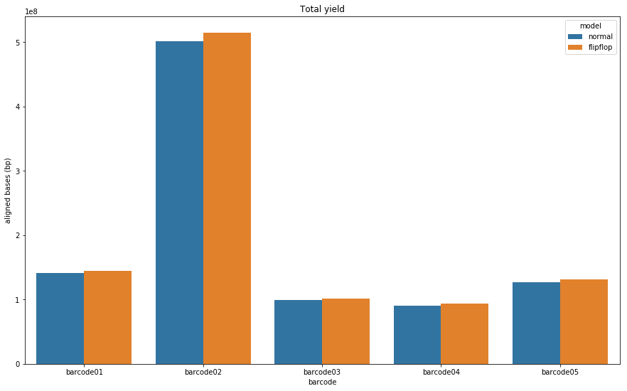 Figure 3: Total number of bases produced by the Guppy default (blue) and flip-flop (orange) algorithms for each barcode.
As you can see. Flip-flop consistently produces more bases. The impact of this will be seen when we look at the relative read lengths for both algorithms.
GC content
As mentioned earlier, M. tuberculosis has a GC content around 65%. Will this have an impact on the new basecaller as Keith Robison seemed to suspect?
sns.set_style("whitegrid")
fig, ax = plt.subplots(figsize=(15, 9))
p = sns.violinplot(x='barcode', y='gc_content', data=df, split=True, inner="quartile",
                   hue='model', hue_order=['normal', 'flipflop'], ax=ax)
p = p.set(title="GC content", ylabel="GC proportion per read (%)")
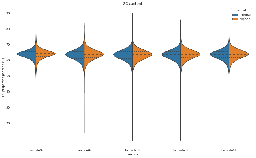 Figure 4: GC content for each barcode calculated on a per-read basis for both the default (blue) and flip-flop (orange) algorithms of Guppy.
I plotted this many different ways and the distributions were nearly identical every way I looked at it. So I guess the flip-flop algorithm may have changed a bit since Keith looked at it, or potentially ONT has some M. tuberculosis in there training dataset?
Read identity
This is the plot I was most interested in. For me, this is the most important plot. How identical are the reads to the section of the reference they map to? As I mentioned already, we don’t have absolute truth here, but it is a pretty close approximation. This metric is effectively asking for the reads that align (I ignore unmapped reads and secondary/supplementary alignments), how similar is the sequence to the reference at that location? I have cut off the axis at 50% to get a clearer view of the bulk of the distribution, but the tails extend past 50%.
sns.set_style("whitegrid")
fig, ax = plt.subplots(figsize=(15, 9))
p = sns.violinplot(y='barcode', x='pid', data=df, split=True, inner="quartile",
                   hue='model', hue_order=['normal', 'flipflop'], ax=ax)
p = p.set(title="Read identity", ylabel="Read percent identity (%)")
_ = ax.set_xlim((50, 100))
_ = plt.legend(loc='lower right')
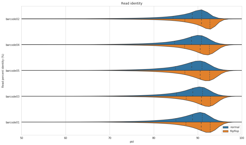 Figure 5: Read percent identity for primary alignments to the M. tuberculosis reference, NC_000962.3. Blue shows the default algorithm for Guppy and orange shows the flip-flop algorithm. The dashed lines within the violins show the percentiles of the data.
Wow! That is a pretty good improvement. On average, flip-flop has about 2% higher read identity compared to Guppy’s default algorithm.
Relative read length
To see whether the algorithms are causing insertions and/or deletions we can look at the relative read length. That is, we take the length of the aligned part of the read and divide it by the length of the aligned part of the reference. Below 1.0 means there have been some deletions, above 1.0 means we’ve had some insertions - compared to the reference of course.
sns.set_style("whitegrid")
fig, ax = plt.subplots(figsize=(15, 9))
p = sns.violinplot(x='barcode', y='rel_len', data=df, split=True, inner="quartile",
                   hue='model', hue_order=['normal', 'flipflop'], ax=ax)
p = p.set(title="Relative read length", ylabel="read alignment length / ref alignment length")
_ = ax.set_ylim((0.75, 1.25))
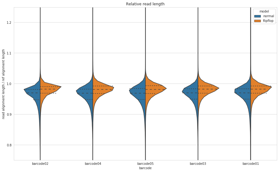 Figure 6: Relative read length for Guppy’s default (blue) and flip-flop (orange) algorithms. Relative read length is calculated as the length of the aligned part of the read and divide it by the length of the aligned part of the reference.
So it appears that flip-flop, on average, causes more deletions than insertions, but it is definitely an improvement on the default algorithm. As we saw from the total yield plot, flip-flop produces more bases and the outcome of that, at least for M. tuberculosis in the case, is fewer deletions.
Conclusions
So in conclusion, given the results from Ryan Wick on S. maltophilia and those presented here on M. tuberculosis, you can make a strong argument for using the flip-flop algorithm over the default for GC-rich genomes without much concern regarding accuracy. You get more accurate reads with fewer deletions. But the big caveat is time. Flip-flop is much slower than the default algorithm. At least on CPUs, it is probably only feasible to use flip-flop if you have a computing cluster with at least 16 cores you can grab unless you want to smash your laptop for a week or so. As I said earlier, I have not been able to run Guppy on GPUs yet, so I am interested to see how much faster flip-flop GPU is compared to the CPU version.
I hope someone finds this useful. And of course, if you have any problems with anything I have done please do get in touch.
Supplementary code
This code was used for preparing the data for plotting.
import pysam
from pathlib import Path
from collections import Counter
import pandas as pd

def gc_content(sequence, as_decimal=True):
    """Returns the GC content for the sequence.
    Notes:
        This method ignores N when calculating the length of the sequence.
        It does not however, ignore other ambiguous bases. It also only
        includes the ambiguous base S (G or C). In this sense, the method is
        conservative with its calculation.
    Args:
        sequence (str): A DNA string.
        as_decimal (bool): Return the result as a decimal. Setting to False
        will return as a percentage. i.e for the sequence GCAT it will
        return 0.5 by default and 50.00 if set to False.
    Returns:
        float: GC content calculated as the number of G, C, and S divided
        by the number of (non-N) bases (length).
    """
    gc_total = 0.0
    num_bases = 0.0
    n_tuple = tuple('nN')
    accepted_bases = tuple('cCgGsS')

    # counter sums all unique characters in sequence. Case insensitive.
    for base, count in Counter(sequence).items():

        # dont count N in the number of bases
        if base not in n_tuple:
            num_bases += count

            if base in accepted_bases:  # S is a G or C
                gc_total += count

    result = gc_total / num_bases

    if not as_decimal:  # return as percentage
        result *= 100

    return result

def get_percent_identity(read):
    """Calculates the percent identity of a read based on the NM tag if present
    , if not calculate from MD tag and CIGAR string.
    Args:
        read (pysam.AlignedSegment): A pysam read alignment record.
    Returns:
        The percent identity or None if required fields are not present.
    """
    try:
        return 100 * (1 - read.get_tag("NM") / read.query_alignment_length)
    except KeyError:
        try:
            return 100 * (
                    1 - (_parse_md_flag(read.get_tag("MD")) +
                         _parse_cigar(read.cigartuples)) /
                    read.query_alignment_length
            )
        except KeyError:
            return None
    except ZeroDivisionError:
        return None

def relative_read_length(read):
    """Calculates the relative read length of the given read.
    That is, read aligned length/reference aligned length.

    Args:
        read (pysam.AlignedSegment): A pysam read alignment record.

    Returns:
        Relative read length as a float.

    """
    return read.query_alignment_length / read.reference_length

def sam_read_stats(filepath):
    """Opens a SAM/BAM file and extracts the read percent identity for all
    mapped reads that are not supplementary or secondary alignments.
    Args:
        filepath (Path): Path to SAM/BAM file.
    Returns:
        A pandas dataframe where the index column is the read id:
            1. 'pid' - read percent identity.
            2. 'rel_len' - relative read length.
            3. 'aligned_bases' - length of query aligned segment.
    """
    # get pysam read option depending on whether file is sam or bam
    file_ext = filepath.suffix
    read_opt = 'rb' if file_ext == '.bam' else 'r'

    # open file
    samfile = pysam.AlignmentFile(filepath, read_opt)

    stats = dict()
    for record in samfile:
        # make sure read is mapped, and is not a suppl. or secondary alignment
        if (record.is_unmapped or
                record.is_supplementary or
                record.is_secondary):
            continue
        pid = get_percent_identity(record)
        relative_len = relative_read_length(record)

        stats[record.query_name] = {
            "pid": pid,
            "rel_len": relative_len,
            "aligned_bases": record.query_alignment_length,
            "gc_content": gc_content(record.query_sequence, as_decimal=False)
        }

    df = pd.DataFrame(stats).T
    df["read_id"] = df.index
    df.reset_index(inplace=True, drop=True)
    return df

def stats_for_bams(bams):
    """Collates stats for a given list of {s,b}am files.
    Args:
        bams (list[Path]): A list of Path objects for {s,b}am files.
    Returns:
        A pandas dataframe of BAM stats where each row is a read and
        the columns are:
            1. 'model' - guppy basecaller model used.
            2. 'barcode' - nanopore barcode.
            3. 'pid' - read percent identity.
            4. 'rel_len' - relative read length.
            5. 'aligned_bases' - length of query aligned segment.
    """
    stats = []
    for bam in bams:
        barcode = bam.name.split('.')[0]
        df = sam_read_stats(bam)
        df['barcode'] = barcode
        stats.append(df)
    return pd.concat(stats)